I randomly came to scikit-learn LogisticRegression page and found they might support different regularization terms such as $\ell$-1 norm, squared $\ell$-2, or their combination. But the constraint is pretty strict/harsh that most cases require $\ell$-1 ratio to be 0, meaning when the objective is non-smooth, many existing solvers don’t work, except SAGA. Besides, to my best knowledge, SAGA requires the regularization term to be convex, which means it is not applicable to nonconvex term such as $\ell$-0 norm. SVRG is an alternative, it is not listed for solving the problem, but SVRG requires the objective to be strongly convex, vanilla LR doesn’t satisfy that. I am a little surprised and not satisfied with the existing solvers and spent time on this problem with interesting findings. In this blog, I would love to share my two cents.
\[\newcommand{\xm}{\mathbf{X}} \newcommand{\fm}{\mathbf{F}} \newcommand{\gm}{\mathbf{G}} \newcommand{\sm}{\mathbf{S}} \newcommand{\um}{\mathbf{U}} \newcommand{\am}{\mathbf{A}} \newcommand{\ym}{\mathbf{Y}} \newcommand{\zm}{\mathbf{Z}} \newcommand{\vx}{\mathbf{x}} \newcommand{\vf}{\mathbf{f}} \newcommand{\vg}{\mathbf{g}} \newcommand{\vq}{\mathbf{q}} \newcommand{\vu}{\mathbf{u}} \newcommand{\vv}{\mathbf{v}} \newcommand{\va}{\mathbf{a}} \newcommand{\vw}{\mathbf{w}} \newcommand{\ve}{\mathbf{e}} \newcommand{\vz}{\mathbf{0}} \newcommand{\rank}{\operatorname{rank}} \newcommand{\Tr}{\operatorname{Tr}} \newcommand{\relint}{\operatorname{relint}} \newcommand{\prox}{\operatorname{prox}} \newcommand{\SVT}{\operatorname{SVT}} \newcommand{\Phiobj}{\Phi} \newcommand{\Domega}{D_{\omega}} \newcommand{\norm}[1]{\left\|#1\right\|} \newcommand{\inner}[2]{\left\langle #1,#2 \right\rangle} \newcommand{\pos}[1]{\left[#1\right]_+}\]Binary Logistic Regression
To begin, we will start with simple LR where the label $y_i$ is $\lbrace -1,1\rbrace$. The objective can be formulated with
\[\min_{\vw} \sum_i\log(1+\exp(-y_i\vx_i^\top\vw)).\]When the label becomes $\lbrace 0,1\rbrace$, the objective changes, but they are essentially equivalent. One should keep in mind that in the above equation, when the lable $y_i$ is different from the sign of $\vx_i^\top\vw$, then $\log$ function will output error. We can define matching score as $y_i\vx_i^\top\vw$: if it is very wrong (magnitude is large, with negative sign), then $\exp$ function will be large; whileas it is very correct (magnitude is large, with positive sign), $\exp$ function will be very small and $\log$ would be almost 0. This is the idea of smoothing $\lbrace 0,1\rbrace$ loss for classification task.
Readers may ask since there are two classes, there should be 2 $\vw$’s: one is $\vw_0$ while the other is $\vw_1$. Indeed, this is reasonable. However, to determine which class a sample belongs to, given the fact $\exp{t}$ is always positive for any $t$, it boils down to check the ratio is larger than 1 or not:
\[\exp\{\vw_0^\top\vx\}/\exp\{\vw_1^\top\vx\}=\exp\{(\vw_0-\vw_1)^\top\vx\}\]Thus the first equation is indeed to set $\vw=\vw_0-\vw_1$.
We call the above observation as shift invariant. In fact, this is somewhat similar to the fact that to seperate two objects, you only need one barrior.
From Binary to Multinomial LR (MLR)
Though Binary case is most fundamental, in real world, multiclassification task is everywhere. One can definitely use the idea of One-VS-One or One-VS-Rest to assign labels, however, this will make the things a lit-bit messier (from my perspective). To allieviate that, MLR is introduced which formulates the objective as
\[\begin{aligned} &L(\mathbf{w}_1,\mathbf{w}_2,\dots,\mathbf{w}_{K-1})\\ =& -\sum_{i=1}^n \log \frac{\exp(\mathbf{w}_{y_i}^T\mathbf{x}_i)} {1+\sum_{l=1}^{K-1}\exp(\mathbf{w}_l^T\mathbf{x}_i)} \\ =& \sum_{i=1}^n \left[ \log\left( 1+\sum_{l=1}^{K-1}\exp(\mathbf{w}_l^T\mathbf{x}_i) \right) - \mathbf{w}_{y_i}^T\mathbf{x}_i \right], \end{aligned}\]if we simply fix $\vw_K=\vz$ for sake of shift invariance.
Apparently,
\[\begin{aligned} \frac{\partial L}{\partial \mathbf{w}_k} &= -\sum_{i=1}^n \left[ \mathbf{1}_{y_i=k} - \frac{\exp(\mathbf{w}_k^T\mathbf{x}_i)} {1+\sum_{l=1}^{K-1}\exp(\mathbf{w}_l^T\mathbf{x}_i)} \right]\mathbf{x}_i, \\ \frac{\partial^2 L}{\partial \mathbf{w}_k^2} &= \sum_{i=1}^n p_i^k(1-p_i^k)\mathbf{x}_i\mathbf{x}_i^T, \end{aligned}\]where we define
\[p_i^k := \frac{\exp(\mathbf{w}_k^T\mathbf{x}_i)} {1+\sum_{l=1}^{K-1}\exp(\mathbf{w}_l^T\mathbf{x}_i)}.\]Thus, we can bound the Lipschitz constant of the gradient by
\[\begin{aligned} \sigma_{\max}\left(\frac{\partial^2 L}{\partial \mathbf{w}_k^2}\right) &= \max_{\|\mathbf{v}\|=1} \mathbf{v}^T \frac{\partial^2 L}{\partial \mathbf{w}_k^2} \mathbf{v} \\ &= \sum_{i=1}^n (\mathbf{v}^*)^T p_i^k(1-p_i^k) \mathbf{x}_i\mathbf{x}_i^T \mathbf{v}^* \\ &\le \frac{1}{4} \sum_{i=1}^n (\mathbf{v}^*)^T \mathbf{x}_i\mathbf{x}_i^T \mathbf{v}^* \\ &= \frac{1}{4} (\mathbf{v}^*)^T \mathbf{X}\mathbf{X}^T \mathbf{v}^* \\ &\le \frac{1}{4} \|\mathbf{X}\|_2^2. \end{aligned}\]This suggests that if we wish, we could update $\vw_0,\dots,\vw_{K-1}$ one by one via gradient descent or proximal GD whereas regularization term exists, with safe stepsize $4/\lVert\mathbf{X}\rVert_2^2$.
On the other side, after tedious arithmetic calculation, we can find the Hessian matrix (class-stacked parameters) $\mathbf{H}\in\mathbb{R}^{d(K-1)\times d(K-1)}$ is
\[\mathbf{H} = \sum_{i=1}^n \left( \operatorname{diag}(\mathbf{p}_i) - \mathbf{p}_i\mathbf{p}_i^\top \right) \otimes \left( \mathbf{x}_i\mathbf{x}_i^\top \right).\]Therefore,
\[\|\mathbf{H}\|_2 \le \frac{1}{2} \left\| \sum_{i=1}^n \mathbf{x}_i\mathbf{x}_i^\top \right\|_2 = \frac{1}{2} \|\mathbf{X}\mathbf{X}^\top\|_2 = \frac{1}{2} \|\mathbf{X}\|_2^2.\]where the first inequality we make use of the following Lemma.
Lemma 0. For any probability vector $\mathbf{p}$, denote
\[\mathbf{J} = \operatorname{diag}(\mathbf{p}) - \mathbf{p}\mathbf{p}^\top.\]Then
\[\lambda_{\max}(\mathbf{J}) = \max_{\|\mathbf{v}\|_2=1} \operatorname{Var}_{\mathbf{p}}(\mathbf{v}) \le \frac{\left(\max(\mathbf{v})-\min(\mathbf{v})\right)^2}{4} \le \frac{1}{2},\]where the last inequality uses $\lVert\mathbf{v}\rVert_2=1$ together with Popoviciu’s inequality on variances (equation attained when $\vv=[\sqrt{2}/2,-\sqrt{2}/2,0,\dots,0]$).
The above conclusion suggests that if we update all $\textbf{W}$’s as a whole, a safe stepsize can be $2/\lVert\mathbf{X}\rVert_2^2$. However, either updating as a whole or block-wise (class by class), we need calculate the spectral norm of $\xm$, which is costly when the data matrix size is huge.
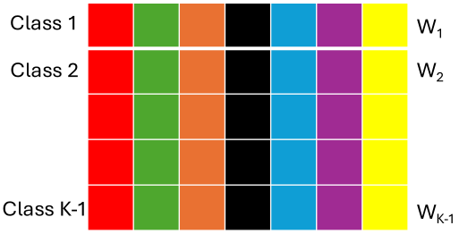
Feature-wise Update
Accordingly, the feature-by-feature block $\mathbf{H}_{rs}$ is given by
\[\mathbf{H}_{rs} = \sum_{i=1}^n x_{ir}x_{is} \left( \operatorname{diag}(\mathbf{p}_i) - \mathbf{p}_i\mathbf{p}_i^\top \right) \in \mathbb{R}^{(K-1)\times(K-1)}.\]Specifically, to update the $s$-th feature block, we need to bound the spectral norm of
\[\mathbf{H}_{ss} = \sum_{i=1}^n x_{is}^2 \left( \operatorname{diag}(\mathbf{p}_i) - \mathbf{p}_i\mathbf{p}_i^\top \right).\]Denote
\[\mathbf{J}_i = \operatorname{diag}(\mathbf{p}_i) - \mathbf{p}_i\mathbf{p}_i^\top.\]Since $\mathbf{H}_{ss}$ is symmetric positive semidefinite, we have
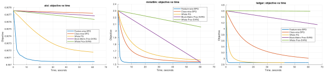
\[\begin{aligned} \|\mathbf{H}_{ss}\|_2 &= \lambda_{\max}(\mathbf{H}_{ss}) \\ &\le \sum_{i=1}^n x_{is}^2 \|\mathbf{J}_i\|_2 \\ &= \sum_{i=1}^n x_{is}^2 \lambda_{\max}(\mathbf{J}_i) \\&\le\frac{\|\xm(:,s)\|_2^2}{2} . \end{aligned}\]The above inequation suggests that we can also update feature wise for matrix $\textbf{W}$, where each feature’s stepsize is determined by $2/\lVert\xm(:,s)\rVert_2^2$. This is critically different as the options aforementioned as no spectral norm is needed, instead, it is to measure the (squared) Euclidean norm of $s$-th column of matrix $\xm$, which is way more cheaper.
A direct by-product and conclusion from the above observation is if data is pre-processed with unit norm, then the stepsize is simply 2 for each feature.
Block Proximal Gradient Method
We will provide different options to determine the order of block to be updated. In the cyclic block proximal gradient (CBPG) method, we successively select a block in a cyclic manner and perform a proximal-gradient step with respect to the chosen block. The $t$-th iterate is denoted by
\[\mathbf{W}_t = \left( \mathbf{w}_t^1, \mathbf{w}_t^2, \dots, \mathbf{w}_t^d \right).\]Each iteration of the CBPG method involves $d$ subiterations. The intermediate iterates generated by these subiterations are denoted by the following auxiliary sequence:
\[\begin{aligned} \mathbf{W}_{t,0} &= \mathbf{W}_t = \left( \mathbf{w}_t^1, \mathbf{w}_t^2, \dots, \mathbf{w}_t^d \right), \\ \mathbf{W}_{t,1} &= \left( \mathbf{w}_{t+1}^1, \mathbf{w}_t^2, \dots, \mathbf{w}_t^d \right), \\ &\quad \vdots \\ \mathbf{W}_{t,d} &= \left( \mathbf{w}_{t+1}^1, \mathbf{w}_{t+1}^2, \dots, \mathbf{w}_{t+1}^d \right). \end{aligned}\]Following the notation above, we have
\[\mathbf{W}_{t,i-1}^i = \mathbf{W}_t^i = \mathbf{w}_t^i,\]and
\[\mathbf{W}_{t,i}^i = \mathbf{W}_{t+1}^i = \mathbf{w}_{t+1}^i.\]Denote
\[\mathbf{W} = (\mathbf{w}^1,\mathbf{w}^2,\dots,\mathbf{w}^d),\] \[\mathcal{U}_i(\mathbf{v}) = \left( \mathbf{0}, \dots, \mathbf{0}, \underbrace{\mathbf{v}}_{i\text{-th block}}, \mathbf{0}, \dots, \mathbf{0} \right),\]and
\[\nabla f(\mathbf{W}) = \left( \nabla_1 f(\mathbf{W}), \nabla_2 f(\mathbf{W}), \dots, \nabla_d f(\mathbf{W}) \right),\]we present the CBPG algorithm as below:
Algorithm: Cyclic Block Proximal Gradient (CBPG) Method
Require:
$\mathbf{X} \in \mathbb{R}^{n \times d}$; initial
$\mathbf{W}_0 = [\mathbf{w}_0^1,\mathbf{w}_0^2,\dots,\mathbf{w}_0^d]$; compute
set $T$, and $t=0$.
For $t \le T$:
-
Set
\[\mathbf{W}_{t,0} \gets \mathbf{W}_t.\] -
For $i=1,\ldots,d$:
\[\mathbf{W}_{t,i} \gets \mathbf{W}_{t,i-1} + \mathcal{U}_i \left( \operatorname{prox}_{\frac{1}{L_i}g_i} \left( \mathbf{W}_{t,i-1}^i - \frac{1}{L_i} \nabla_i f(\mathbf{W}_{t,i-1}) \right) - \mathbf{W}_{t,i-1}^i \right).\] -
Set
\[\mathbf{W}_{t+1} \gets \mathbf{W}_{t,d}.\]
We now establish a convergence rate in terms of function values for the CBPG method in the MLR setting, where $f$ is convex, $L_f$-smooth and a certain boundedness property of the level sets of $F$ holds; see Beck (2017).
Assumption 1 For any $\alpha>0$, there exists $R_\alpha>0$ such that
\[\max_{\mathbf{x},\mathbf{x}^*} \left\{ \|\mathbf{x}-\mathbf{x}^*\| : F(\mathbf{x})\le \alpha \right\} \le R_\alpha.\]Lemma 1 Let $\lbrace \mathbf{W}_t\rbrace$ be the sequence generated by the CBPG method described in the algorithm for solving the optimization problem. Then, for any $t\ge 0$,
\[F(\mathbf{W}_t)-F(\mathbf{W}_{t+1}) \ge \frac{L_{\min}} {2d(L_f+L_{\max})^2R^2} \left( F(\mathbf{W}_{t+1})-F_{\mathrm{opt}} \right),\]where
\[R=R_{F(\mathbf{W}_0)}, \qquad L_{\max}=\max_{j=1,2,\dots,d} L_j, \qquad L_{\min}=\min_{j=1,2,\dots,d} L_j.\]Theorem 1 ($\mathcal{O}(1/t)$ rate of convergence of CBPG) Suppose that the boundedness assumption holds. Let $\lbrace\mathbf{W}_t\rbrace$ be the sequence generated by the CBPG method for solving the optimization problem. Then, for any $t\ge 2$,
\[\begin{aligned} F(\mathbf{W}_t)-F_{\mathrm{opt}} \le \max\Bigg\{ &\left(\frac{1}{2}\right)^{(t-1)/2} \left(F(\mathbf{W}_0)-F_{\mathrm{opt}}\right), \\ &\frac{ 8d(L_{\max}+L_f)^2R^2 }{ L_{\min}(t-1) } \Bigg\}. \end{aligned}\]In addition, if $t\ge 2$ satisfies
\[t \ge 1+ \max\Bigg\{ \frac{2}{\log 2} \left( \log\left(F(\mathbf{W}_0)-F_{\mathrm{opt}}\right) + \log\frac{1}{\epsilon} \right), \; \frac{ 8d(L_{\max}+L_f)^2R^2 }{ L_{\min}\epsilon } \Bigg\},\]then
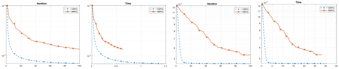
\[F(\mathbf{W}_t)-F_{\mathrm{opt}} \le \epsilon.\]The analysis of the CBPG method was done under the assumption that the index selection strategy is cyclic. We now introduce a version of the block proximal gradient method, in which at each iteration, a prox-grad step is performed at a randomly chosen block. Similar to CBPG, the randomized method is also monotonically decreasing while the difference is that in each loop, only a random block will be updated instead of each.
Algorithm: Randomized Block Proximal Gradient (RBPG) Method
Require:
$\mathbf{X}\in\mathbb{R}^{n\times d}$; initial point
compute
\[L_i=\frac{\lVert\xm(:,i)\rVert_2^2}{2},\]set $T$, and initialize $t=0$.
For $t\le T$:
-
Sample
\[i_t\in\{1,2,\dots,d\}\]uniformly at random.
-
Update
\[\mathbf{W}_{t+1} \gets \mathbf{W}_t + \mathcal{U}_{i_t} \left( \operatorname{prox}_{\frac{1}{L_{i_t}}g_{i_t}} \left( \mathbf{w}_t^{i_t} - \frac{1}{L_{i_t}} \nabla_{i_t}f(\mathbf{W}_t) \right) - \mathbf{w}_t^{i_t} \right).\]
Theorem 2 ($\mathcal{O}(1/t)$ rate of convergence of RBPG) Let $\lbrace\mathbf{W}_t\rbrace$ be the sequence generated by the RBPG method for solving the optimization problem. For any $t\ge 0$, define
\[\|\mathbf{W}\|_L^2 := \sum_{i=1}^d L_i\|\mathbf{w}^i\|_2^2.\]Then
\[\begin{aligned} \mathbb{E}_{\xi_t} \left[ F(\mathbf{W}_{t+1}) \right] - F_{\mathrm{opt}} \le \frac{d}{d+t+1} \left( \frac{1}{2} \|\mathbf{W}_0-\mathbf{W}_*\|_L^2 + F(\mathbf{W}_0)-F_{\mathrm{opt}} \right). \end{aligned}\]Apparently, the above theorem suggests that when $d$ is smaller, it converges faster.
For the sake of simplicity, the reader may find proof in the paper for details.
Experiments
References
[1] Kevin Murphy. “Probabilistic Machine Learning: An Introduction.” MIT Press, 2022.
[2] Amir Beck. “First-order methods in optimization”.