Tensor completion asks us to recover a multidimensional array from only a subset of its entries. A hyperspectral image is indexed by height, width, and wavelength. A grayscale video adds time as a third mode, while a color video is naturally fourth-order. Traffic measurements, medical scans, recommendation data, and spatiotemporal sensor streams have the same structure: the observations are multidimensional, incomplete, and highly correlated.
Let
\[\mathcal{Y} \in \mathbb{R}^{I_1\times I_2\times\cdots\times I_N}\]be a partially observed tensor, let $\Omega$ be the set of observed indices, and let $P_\Omega$ keep entries in $\Omega$ while setting all other entries to zero. The goal is to find a tensor $\mathcal{X}$ that agrees with the observed data and has low-rank structure.
The matrix version of this problem has a clean convex model based on the nuclear norm. The tensor version is harder. Tensor rank is not uniquely defined, there is no universal tensor SVD, and many basic tensor spectral problems are NP-hard. Penalizing the nuclear norms of mode unfoldings is tractable, but repeatedly decomposing those large matrices can dominate runtime and memory.
We study an SVD-free alternative built from four ideas:
- represent the recovered tensor with one coupled canonical polyadic decomposition,
- use every mode to construct a factor regularizer that upper-bounds the atomic tensor nuclear norm,
- separate the looseness of that bound into decomposition and factor-scaling gaps,
- optimize the factor blocks cyclically by exact linear solves or gradient steps.
The resulting objective is jointly nonconvex but quadratic, smooth, and strongly convex in each factor block. This structure gives monotonic descent, convergence to a stationary point, and an $O(1/K)$ rate for the minimum squared stationarity measure. The experiments evaluate the method under extreme missingness, observation noise, matched wall-clock budgets, and increasing tensor size, order, rank, and observation count.
From Matrix Completion to Tensor Completion
It is useful to begin with the matrix problem. Given a partially observed matrix $\mathbf{Y}$, nuclear-norm-regularized matrix completion solves
\[\min_{\mathbf{X}} \quad \frac{1}{2} \|P_\Omega(\mathbf{X}-\mathbf{Y})\|_F^2 + \lambda\|\mathbf{X}\|_*.\]The first term fits the observed entries. The nuclear norm
\[\|\mathbf{X}\|_* = \sum_j\sigma_j(\mathbf{X})\]is the sum of the singular values and is the standard convex surrogate for matrix rank. Its computational weakness is that a proximal step requires singular value thresholding, which in turn requires an SVD.
The key variational identity is
\[\|\mathbf{X}\|_* = \min_{\mathbf{A}\mathbf{B}^{\top}=\mathbf{X}} \frac{1}{2} \left( \|\mathbf{A}\|_F^2 + \|\mathbf{B}\|_F^2 \right).\]If $\mathbf{X}=\mathbf{U}\mathbf{\Sigma}\mathbf{V}^{\top}$ is an SVD, the minimum is attained by
\[\mathbf{A} = \mathbf{U}\mathbf{\Sigma}^{1/2}, \qquad \mathbf{B} = \mathbf{V}\mathbf{\Sigma}^{1/2}.\]Therefore the matrix problem can be written in the Burer–Monteiro form
\[\min_{\mathbf{A},\mathbf{B}} \quad \frac{1}{2} \|P_\Omega(\mathbf{A}\mathbf{B}^{\top}-\mathbf{Y})\|_F^2 + \frac{\lambda}{2} \left( \|\mathbf{A}\|_F^2 + \|\mathbf{B}\|_F^2 \right).\]Once the factor width is at least the rank of an optimal solution, the factorized problem and the nuclear-norm problem have the same optimal value. The important computational change is that we optimize thin factors instead of repeatedly decomposing a large completed matrix.
The tensor method begins with this identity and applies it to all mode unfoldings through one shared CP factorization.
CP Decomposition and Mode Unfoldings
For an $N$th-order tensor
\[\mathcal{X} \in \mathbb{R}^{I_1\times\cdots\times I_N},\]a rank-$R$ canonical polyadic, or CP, decomposition is
\[\mathcal{X} = \sum_{r=1}^{R} \boldsymbol{a}_{1,r} \circ \boldsymbol{a}_{2,r} \circ\cdots\circ \boldsymbol{a}_{N,r}.\]Here $\circ$ denotes the vector outer product. Collecting the vectors for each mode gives
\[\mathbf{A}_i = [\boldsymbol{a}_{i,1},\ldots,\boldsymbol{a}_{i,R}] \in \mathbb{R}^{I_i\times R},\]and we write
\[\mathcal{X} = [[\mathbf{A}_1,\ldots,\mathbf{A}_N]].\]The mode-$i$ unfolding $\mathbf{X}_{(i)}$ arranges the mode-$i$ fibers as columns of a matrix. Under the CP model,
\[\mathbf{X}_{(i)} = \mathbf{A}_i\mathbf{B}_i^{\top},\]where
\[\mathbf{B}_i = \mathbf{A}_N \odot\cdots\odot \mathbf{A}_{i+1} \odot \mathbf{A}_{i-1} \odot\cdots\odot \mathbf{A}_1\]and $\odot$ denotes the Khatri–Rao product. Its dimensions are
\[\mathbf{B}_i \in \mathbb{R}^{(\prod_{j\neq i}I_j)\times R}.\]This is the bridge from matrix to tensor completion. Every unfolding is a matrix product, but all unfoldings share the same CP factors. Unlike methods that maintain an independent factor pair and rank for every unfolding, the model stores one coupled representation with one target rank.
An SVD-Free Nuclear-Norm Surrogate
One common tensor regularizer averages the nuclear norms of all mode unfoldings:
\[\|\mathcal{X}\|_{\mathrm{unfold},*} = \frac{1}{N} \sum_{i=1}^{N} \|\mathbf{X}_{(i)}\|_*.\]This gives the completion model
\[\min_{\mathcal{X}} \quad \frac{1}{2} \|P_\Omega(\mathcal{X}-\mathcal{Y})\|_F^2 + \frac{\lambda}{N} \sum_{i=1}^{N} \|\mathbf{X}_{(i)}\|_*.\]For the CP factors, the matrix identity gives
\[\|\mathbf{X}_{(i)}\|_* \leq \frac{1}{2} \left( \|\mathbf{A}_i\|_F^2 + \|\mathbf{B}_i\|_F^2 \right).\]The Khatri–Rao factor does not need to be constructed densely. Its Gram matrix satisfies
\[\mathbf{B}_i^{\top}\mathbf{B}_i = \mathop{*}_{j\neq i} (\mathbf{A}_j^{\top}\mathbf{A}_j),\]where $*$ is the Hadamard product. Consequently,
\[\|\mathbf{B}_i\|_F^2 = \operatorname{tr} \left( \mathop{*}_{j\neq i} (\mathbf{A}_j^{\top}\mathbf{A}_j) \right).\]Define the factor regularizer
\[\mathcal{R}(\mathbf{A}_1,\ldots,\mathbf{A}_N) = \frac{1}{2N} \sum_{i=1}^{N} \left[ \|\mathbf{A}_i\|_F^2 + \operatorname{tr} \left( \mathop{*}_{j\neq i} (\mathbf{A}_j^{\top}\mathbf{A}_j) \right) \right].\]The proposed objective is
\[\begin{aligned} \min_{\mathbf{A}_1,\ldots,\mathbf{A}_N} \quad F(\mathbf{A}_1,\ldots,\mathbf{A}_N) =& \frac{1}{2} \left\| P_\Omega \left( \mathcal{Y} - [[\mathbf{A}_1,\ldots,\mathbf{A}_N]] \right) \right\|_F^2 \\ &+ \lambda \mathcal{R}(\mathbf{A}_1,\ldots,\mathbf{A}_N). \end{aligned}\]This expression uses every mode and contains no tensor or unfolding SVD. It is also an upper bound for the atomic tensor nuclear norm. If
\[\mathcal{X} = \sum_{r=1}^{R} \boldsymbol{v}_{1,r} \circ\cdots\circ \boldsymbol{v}_{N,r},\]set
\[u_{i,r}=\|\boldsymbol{v}_{i,r}\|_2, \qquad \mu_r=\prod_{i=1}^{N}u_{i,r}.\]After normalizing every nonzero factor vector, the $r$th rank-one term has coefficient $\mu_r$. The scalar inequality
\[2u_{i,r} \prod_{j\neq i}u_{j,r} \leq u_{i,r}^2 + \prod_{j\neq i}u_{j,r}^2\]then gives
\[\|\mathcal{X}\|_* \leq \sum_{r=1}^{R}\mu_r \leq \mathcal{R}(\mathbf{A}_1,\ldots,\mathbf{A}_N).\]For matrices, the factor penalty can reproduce the nuclear norm exactly. For higher-order tensors, the shared factors and their scaling generally leave a nonzero gap. The new paper characterizes that gap exactly.
Tightness and Gap Analysis
For each nonzero CP component, write
\[\widehat{\boldsymbol{v}}_{i,r} = \frac{\boldsymbol{v}_{i,r}}{u_{i,r}}, \qquad \|\widehat{\boldsymbol{v}}_{i,r}\|_2=1.\]Then
\[\mathcal{X} = \sum_{r=1}^{R} \mu_r \widehat{\boldsymbol{v}}_{1,r} \circ\cdots\circ \widehat{\boldsymbol{v}}_{N,r}.\]The surrogate has the exact decomposition
\[\begin{aligned} \mathcal{R}(\mathbf{A}_1,\ldots,\mathbf{A}_N) =& \sum_{r=1}^{R}\mu_r \\ &+ \frac{1}{2N} \sum_{r=1}^{R} \sum_{i=1}^{N} \left( u_{i,r} - \prod_{j\neq i}u_{j,r} \right)^2. \end{aligned}\]Subtracting the atomic tensor nuclear norm gives
\[\mathcal{R}(\mathbf{A}_1,\ldots,\mathbf{A}_N) - \|\mathcal{X}\|_* = \Delta_{\mathrm{dec}} + \Delta_{\mathrm{scale}},\]where
\[\Delta_{\mathrm{dec}} = \sum_{r=1}^{R}\mu_r - \|\mathcal{X}\|_* \geq0\]and
\[\Delta_{\mathrm{scale}} = \frac{1}{2N} \sum_{r=1}^{R} \sum_{i=1}^{N} \left( u_{i,r} - \prod_{j\neq i}u_{j,r} \right)^2 \geq0.\]The two terms describe different sources of looseness.
- The decomposition gap asks whether the chosen normalized CP representation is nuclear-norm minimizing. Even perfect factor balancing cannot remove a poor decomposition.
- The scaling gap comes from the quadratic inequality used to build the surrogate. It can be reduced without changing the represented tensor because reciprocal rescaling leaves a CP rank-one component unchanged.
Optimal Scaling of a CP Component
Consider one component with coefficient $\mu>0$. Its factor norms satisfy
\[\prod_{i=1}^{N}u_i=\mu,\]and its contribution to the surrogate is
\[q_N(u_1,\ldots,u_N) = \frac{1}{2N} \sum_{i=1}^{N} \left( u_i^2 + \frac{\mu^2}{u_i^2} \right).\]Among all equivalent scalings, the minimum occurs when the factor norms are balanced:
\[u_1=\cdots=u_N=\mu^{1/N}.\]The corresponding surrogate contribution is
\[\phi_N(\mu) = \frac{1}{2} \left( \mu^{2/N} + \mu^{2-2/N} \right),\]so the smallest possible scaling gap is
\[g_N(\mu) = \phi_N(\mu)-\mu = \frac{1}{2} \left( \mu^{1/N} - \mu^{1-1/N} \right)^2.\]Its relative form is especially revealing:
\[\frac{g_N(\mu)}{\mu} = \cosh \left[ \left(1-\frac{2}{N}\right) \log\mu \right] -1.\]For matrices, $N=2$ and $g_2(\mu)=0$ for every positive $\mu$. This recovers the exact Burer–Monteiro identity. For $N>2$, the balanced scaling gap is zero only when $\mu=1$. Near one,
\[\frac{g_N(\mu)}{\mu} = \frac{1}{2} \left(1-\frac{2}{N}\right)^2 (\log\mu)^2 + O\left((\log\mu)^4\right).\]The surrogate is therefore tight when the logarithms of the CP coefficients are concentrated near zero, and it becomes looser as the tensor order or the coefficient spread grows.
Expected Gap for Random Coefficients
Assume the normalized CP decomposition attains the atomic nuclear norm, the component coefficients are independent copies of a positive random variable $M$, and every component uses balanced scaling. Then
\[\mathbb{E} \left[ \mathcal{R}-\|\mathcal{X}\|_* \right] = R\,\mathbb{E}[g_N(M)],\]with
\[\mathbb{E}[g_N(M)] = \frac{1}{2}\mathbb{E}[M^{2/N}] + \frac{1}{2}\mathbb{E}[M^{2-2/N}] - \mathbb{E}[M].\]For a lognormal coefficient $\log M\sim\mathcal{N}(\eta,\sigma_\mu^2)$, the required moments are explicit. In the centered, small-variance case,
\[\mathbb{E}[g_N(M)] = \frac{1}{2} \left(1-\frac{2}{N}\right)^2 \sigma_\mu^2 + o(\sigma_\mu^2).\]This turns the qualitative upper-bound statement into a quantitative one: coefficient variability and tensor order control the expected scaling gap.
Block Structure and Exact Updates
The full objective is not jointly convex because the CP reconstruction multiplies all factors. If all factors except $\mathbf{A}_i$ are fixed, however, the remaining block problem is a strongly convex quadratic.
Let
\[\boldsymbol{a}_i = \operatorname{vec}(\mathbf{A}_i), \qquad \boldsymbol{y}_i = \operatorname{vec}(\mathbf{Y}_{(i)}),\]and define
\[\mathbf{K}_i = \mathbf{B}_i\otimes\mathbf{I}_{I_i}.\]Let $\mathbf{P}_i$ be the vectorized mode-$i$ observation mask. To express the regularizer, define
\[\mathbf{D}_i = \operatorname{Diag} \left[ \operatorname{diag} \left( \sum_{j\neq i}\mathbf{H}_{i,j} \right) \right],\]where
\[\mathbf{H}_{i,j} = \mathop{*}_{\ell\notin\{i,j\}} (\mathbf{A}_\ell^{\top}\mathbf{A}_\ell), \qquad \mathbf{M}_i = \mathbf{D}_i\otimes\mathbf{I}_{I_i}.\]Up to terms independent of $\boldsymbol{a}_i$, the block objective is
\[\begin{aligned} F_i(\boldsymbol{a}_i;\mathcal{A}_{-i}) =& \frac{1}{2} \left\| \mathbf{P}_i \left( \boldsymbol{y}_i - \mathbf{K}_i\boldsymbol{a}_i \right) \right\|_2^2 \\ &+ \frac{\lambda}{2N} \boldsymbol{a}_i^{\top} \left( \mathbf{I}_{I_iR} + \mathbf{M}_i \right) \boldsymbol{a}_i. \end{aligned}\]Define
\[\mathbf{G}_i = \mathbf{K}_i^{\top} \mathbf{P}_i^{\top}\mathbf{P}_i \mathbf{K}_i + \frac{\lambda}{N} \left( \mathbf{I}_{I_iR} + \mathbf{M}_i \right)\]and
\[\boldsymbol{b}_i = \mathbf{K}_i^{\top} \mathbf{P}_i^{\top}\mathbf{P}_i \boldsymbol{y}_i.\]Then
\[\nabla_iF = \mathbf{G}_i\boldsymbol{a}_i - \boldsymbol{b}_i, \qquad \nabla_{ii}^2F = \mathbf{G}_i.\]Because $\lambda>0$,
\[\mathbf{G}_i \succeq \frac{\lambda}{N} \mathbf{I}_{I_iR}.\]Thus every block is at least $\mu=\lambda/N$ strongly convex and has a unique minimizer. Its exact block Lipschitz constant is
\[L_i^{\mathrm{exact}} = \lambda_{\max}(\mathbf{G}_i).\]A convenient computable upper bound is
\[\widehat{L}_i = \lambda_{\max} \left( \mathop{*}_{\ell\neq i} \mathbf{A}_\ell^{\top}\mathbf{A}_\ell \right) + \frac{\lambda}{N} \left( 1+\|\mathbf{D}_i\|_2 \right).\]This produces two valid block updates.
Exact block minimization. Solve the positive-definite linear system
\[\mathbf{G}_i\boldsymbol{a}_i^+ = \boldsymbol{b}_i.\]The inverse should never be formed explicitly; a positive-definite linear solver computes the unique minimizer.
Block-gradient update. For any $L_i\geq\lambda_{\max}(\mathbf{G}_i)$,
\[\boldsymbol{a}_i^+ = \boldsymbol{a}_i - \frac{1}{L_i} \left( \mathbf{G}_i\boldsymbol{a}_i - \boldsymbol{b}_i \right).\]The exact step is more expensive per sweep but completely solves the current block. The gradient step is cheaper but may require many more sweeps.
Cyclic Block Optimization
The new solver updates factors sequentially and always uses the newest available values. If $\mathcal{A}^k$ denotes the factors at the start of sweep $k$, define
\[\mathcal{A}^{k,i} = \left( \mathbf{A}_1^{k+1},\ldots,\mathbf{A}_i^{k+1}, \mathbf{A}_{i+1}^{k},\ldots,\mathbf{A}_N^{k} \right).\]Thus block $i+1$ immediately sees the newly updated blocks $1$ through $i$.
Algorithm: Cyclic Block Optimization
Input: observed tensor $\mathcal{Y}$, observation set $\Omega$, target rank $R$, regularization $\lambda>0$, and block types $q_i\in{\mathrm{Exact},\mathrm{Gradient}}$
Output: recovered tensor $\widehat{\mathcal{X}}$
-
Initialize
\[\mathcal{A}^0 = (\mathbf{A}_1^0,\ldots,\mathbf{A}_N^0).\] -
For sweeps $k=0,1,2,\ldots$ until convergence:
-
Set $\mathcal{A}^{k,0}=\mathcal{A}^k$.
-
For $i=1,\ldots,N$:
-
Form $\mathbf{B}_i^k$, $\mathbf{K}_i^k$, $\mathbf{D}_i^k$, $\mathbf{G}_i^k$, and $\boldsymbol{b}_i^k$ using $\mathcal{A}^{k,i-1}$.
-
If $q_i=\mathrm{Exact}$, solve
\[\mathbf{G}_i^k \boldsymbol{a}_i^{k+1} = \boldsymbol{b}_i^k.\] -
Otherwise choose $L_i^k\geq\lambda_{\max}(\mathbf{G}_i^k)$ and set
\[\boldsymbol{a}_i^{k+1} = \boldsymbol{a}_i^k - \frac{1}{L_i^k} \left( \mathbf{G}_i^k\boldsymbol{a}_i^k - \boldsymbol{b}_i^k \right).\] -
Reshape $\boldsymbol{a}_i^{k+1}$ into $\mathbf{A}_i^{k+1}$ and update $\mathcal{A}^{k,i}$.
-
-
Set $\mathcal{A}^{k+1}=\mathcal{A}^{k,N}$.
-
-
Return
\[\widehat{\mathcal{X}} = [[\mathbf{A}_1^k,\ldots,\mathbf{A}_N^k]].\]
Choosing exact minimization for every block gives regularized alternating least squares. Choosing gradient steps for every block gives cyclic block-gradient descent. A hybrid can mix the two. The experiments call the all-exact version Cyclic Block Optimization, or CBO, because validation selects exact updates on all five real tensors.
Convergence Analysis
The convergence theorem does not assume that the joint objective is convex, nor does it require a no-spurious-local-minima hypothesis. Suppose $\lambda>0$, every gradient block uses
\[L_i^k \geq \lambda_{\max}(\mathbf{G}_i^k),\]and the selected constants remain uniformly bounded:
\[L_i^k\leq\overline{L}<\infty.\]The computable Lipschitz bound above satisfies this condition on the bounded level set generated by the algorithm.
Let
\[F_{\inf} = \inf_{\mathcal{A}}F(\mathcal{A}), \qquad \mu = \frac{\lambda}{N}.\]Both exact and gradient updates provide sufficient decrease. Summing over one complete sweep gives
\[F(\mathcal{A}^k) - F(\mathcal{A}^{k+1}) \geq \frac{\mu}{2} \|\mathcal{A}^{k+1}-\mathcal{A}^{k}\|^2.\]Because every regularization term is nonnegative,
\[F(\mathcal{A}) \geq \frac{\lambda}{2N} \sum_{i=1}^{N} \|\mathbf{A}_i\|_F^2.\]The objective is coercive, so its initial level set is compact and the iterates are bounded. Telescoping the sufficient-decrease inequality gives
\[\sum_{k=0}^{\infty} \|\mathcal{A}^{k+1}-\mathcal{A}^{k}\|^2 \leq \frac{2}{\mu} \left( F(\mathcal{A}^0)-F_{\inf} \right).\]In particular,
\[\|\mathcal{A}^{k+1}-\mathcal{A}^{k}\| \longrightarrow0.\]For every integer $K\geq1$,
\[\min_{0\leq k<K} \|\mathcal{A}^{k+1}-\mathcal{A}^{k}\|^2 \leq \frac{ 2\left(F(\mathcal{A}^0)-F_{\inf}\right) }{ \mu K }.\]Let $\Lambda$ be a Lipschitz constant for the full gradient on the compact level set. The block optimality conditions relate the final gradient to the sweep displacement, yielding
\[\min_{0\leq k<K} \|\nabla F(\mathcal{A}^{k+1})\|^2 \leq \frac{ 4\left(\overline{L}^2+N\Lambda^2\right) \left(F(\mathcal{A}^0)-F_{\inf}\right) }{ \mu K }.\]Therefore
\[\min_{0\leq k<K} \|\nabla F(\mathcal{A}^{k+1})\| = O(K^{-1/2}),\]or equivalently the minimum squared stationarity measure decays as $O(1/K)$.
Every accumulation point is stationary. Because $F$ is a polynomial in the factor entries, it has the Kurdyka–Lojasiewicz property. Together with sufficient decrease, boundedness, and the relative gradient bound, this implies that the complete sequence converges to one stationary point.
The theorem is a stationary-point result for the nonconvex cyclic method. It covers exact, gradient, and hybrid block updates without assuming that a stationary point is globally optimal.
What the Experiments Show
The evaluation uses five large real tensors.
| Tensor | Modality | Shape | Entries |
|---|---|---|---|
| CAVE Balloons | Hyperspectral image | $256\times256\times31$ | 2.03M |
| Xiph Bus | Grayscale video | $144\times176\times72$ | 1.82M |
| Seattle | Traffic | $323\times28\times288$ | 2.60M |
| Portland | Traffic | $1156\times31\times96$ | 3.44M |
| Xiph City | Color video | $144\times176\times3\times72$ | 5.47M |
Each tensor is min-max normalized to $[0,1]$. The observation masks retain either $20\%$ or $10\%$ of the entries, corresponding to $80\%$ and $90\%$ missingness. Noise is added only to observed entries:
\[Y_\omega = X_\omega + \sigma \left( \max(\mathcal{X})-\min(\mathcal{X}) \right) \epsilon_\omega, \qquad \epsilon_\omega\sim\mathcal{N}(0,1),\]with $\sigma\in{0,0.01,0.05,0.10}$. Evaluation always uses the clean values on the missing set $\mathcal{M}=\Omega^c$:
\[\operatorname{RMSE}_{\mathcal{M}} = \sqrt{ \frac{1}{|\mathcal{M}|} \left\| P_{\mathcal{M}} \left( \widehat{\mathcal{X}}-\mathcal{X} \right) \right\|_F^2 }.\]The baselines are PALM on the same factorized objective, CP-WOPT, HaLRTC, LRTC-TNN, TT-WOPT for the fourth-order video, and LATC for traffic tensors. Mean filling is a non-iterative reference. Hyperparameters are selected on held-out observed entries and then frozen. Every iterative method receives a literal five-second solver budget. The experiments use five shared random masks per condition.
Validation chooses all-exact CBO on every tensor, with $(R,\lambda)=(8,10^{-3})$ for CAVE and $(R,\lambda)=(4,10^{-4})$ for the other four tensors.
Extreme Missingness and Noise
With clean observations, CBO has the lowest mean missing-entry RMSE in nine of the ten dataset-missingness settings.
| Tensor | Missing | CBO RMSE | Best other RMSE | Best other |
|---|---|---|---|---|
| CAVE | 80% | 0.03737 | 0.05306 | HaLRTC |
| CAVE | 90% | 0.03761 | 0.13482 | HaLRTC |
| Bus | 80% | 0.15728 | 0.14022 | HaLRTC |
| Bus | 90% | 0.15660 | 0.17958 | HaLRTC |
| Seattle | 80% | 0.08013 | 0.10278 | HaLRTC |
| Seattle | 90% | 0.07927 | 0.12717 | HaLRTC |
| Portland | 80% | 0.01878 | 0.05069 | HaLRTC |
| Portland | 90% | 0.01913 | 0.05360 | HaLRTC |
| City | 80% | 0.08024 | 0.08209 | TT-WOPT |
| City | 90% | 0.07895 | 0.08181 | TT-WOPT |
Across five datasets, two missingness levels, and four noise levels, CBO wins 36 of 40 condition cells and has mean rank $1.10$. All four losses are the Xiph Bus cases at $80\%$ missingness, where HaLRTC ranks first. At $\sigma=0.10$, CBO’s median RMSE increase relative to clean observations is only $0.44\%$. Portland is the outlier: its increase is $19.85\%$ at $80\%$ missingness and $30.72\%$ at $90\%$, although its absolute RMSE remains below every baseline.
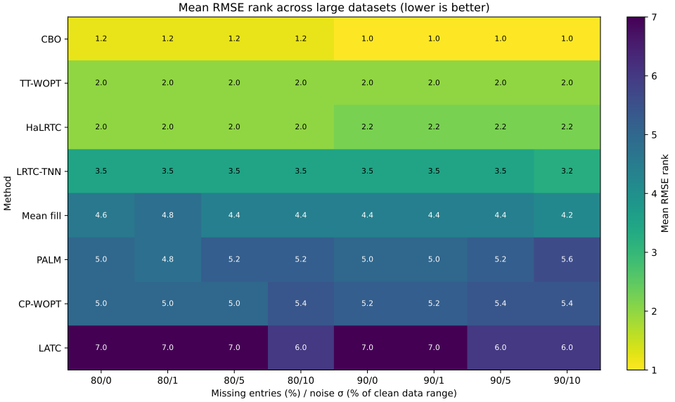
The small difference between $80\%$ and $90\%$ missingness for some factorized methods is a wall-clock effect. Fewer observations make each sweep cheaper, so the solver completes more sweeps within the same five seconds.
Cyclic Update Ablation
The optimizer ablation holds the model, observations, rank, regularization, and initial factors fixed. It compares exact cyclic updates, Lipschitz-gradient cyclic updates, a hybrid, and PALM on a smaller CAVE tensor and fourth-order City video.
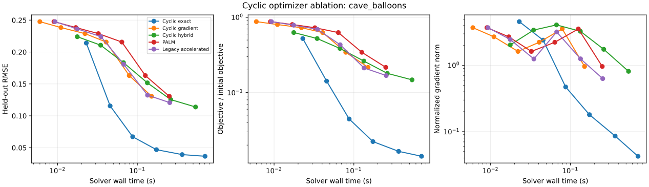
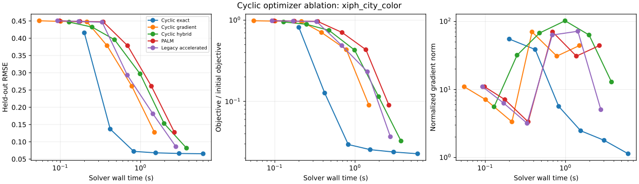
At 32 sweeps, the results are:
| Optimizer | CAVE RMSE / s | City RMSE / s |
|---|---|---|
| Exact cyclic | 0.0366 / 0.706 | 0.0654 / 6.025 |
| Gradient cyclic | 0.1306 / 0.151 | 0.1274 / 1.490 |
| Hybrid cyclic | 0.1138 / 0.537 | 0.0816 / 3.739 |
| PALM | 0.1306 / 0.251 | 0.1274 / 2.641 |
Exact updates cost more per sweep, but by the final checkpoint they reach substantially lower error, objective, and stationarity. Across all 300 ablation trajectories, no objective increase exceeds numerical tolerance, matching the monotonic-descent theorem.
Accuracy Versus Wall Time
The five-second table shows one operating point. The time-accuracy experiment repeats deterministic fits at nominal budgets from one to ten seconds and plots RMSE against the actual median solver time.
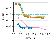
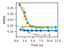
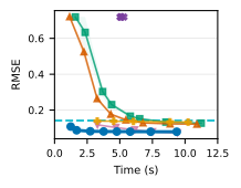
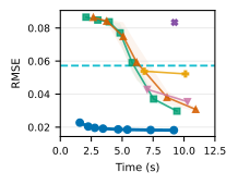
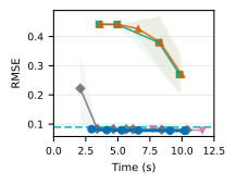

Among the 38 dataset-budget cells with at least one iterative method inside the predeclared timing window, CBO obtains the lowest mean RMSE in 26. HaLRTC wins nine; PALM, CP-WOPT, and TT-WOPT each win one. The curves also show that no single method dominates at every horizon: CBO improves quickly, while HaLRTC crosses it later on CAVE, Bus, and Seattle.
Scalability
The scaling study generates sparse observations directly from CP factors without materializing the dense tensor. It varies order in ${3,4,5}$, total entries from roughly $1.3\times10^5$ to $8.5\times10^6$, rank from $4$ to $32$, and observation rate from $5\%$ to $40\%$.
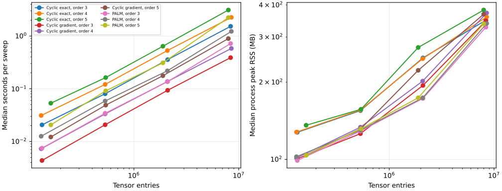
Exact cyclic time grows nearly linearly with the number of tensor entries: the empirical exponents are $1.043$, $1.031$, and $1.049$ for orders three, four, and five. At the largest tested sizes, one exact sweep takes $1.53$, $2.26$, and $3.12$ seconds, with peak memory of $349$, $359$, and $382$ MB.
Rank is the main cost driver for exact solves. On a 2.10-million-entry third-order tensor with $10\%$ observations, increasing $R$ from $4$ to $32$ raises time from $0.211$ to $8.689$ seconds per sweep and memory from $165$ to $1162$ MB. At rank eight, increasing the observation rate from $5\%$ to $40\%$ raises time from $0.249$ to $2.730$ seconds. All 180 scaling fits remain numerically monotone.
Takeaways
The main modeling lesson is that low-rank tensor completion does not require a monolithic tensor SVD or a separate factorization for every unfolding. A CP representation turns each mode unfolding into a matrix product, and the matrix nuclear-norm identity yields one coupled, SVD-free factor regularizer.
The new gap analysis makes the approximation precise. The total looseness is the sum of a decomposition gap and a scaling gap. Balancing each rank-one component minimizes the scaling contribution, recovers exactness for matrices, and shows why higher tensor order and more variable CP coefficients make the surrogate less tight.
The main optimization lesson is that cyclic block optimization can exploit the objective structure directly. Every block is a strongly convex quadratic, so it can be solved exactly by a positive-definite linear system or advanced by a valid gradient step. Exact cyclic updates are more expensive per sweep but decisively outperform the cheaper updates in the ablation.
The convergence guarantee is a nonconvex stationary-point result: monotonic descent, bounded and square-summable steps, convergence of the full sequence, and an $O(1/K)$ rate for the minimum squared gradient norm. It does not claim that every stationary point is globally optimal.
Finally, the experiments make the computational trade-off visible. CBO is accurate under 80-90% missingness and substantial observation noise, works on third- and fourth-order real tensors, and scales nearly linearly with the number of entries. Its main limitation is rank: exact block systems become substantially more expensive as $R$ grows.
References
- Frank L. Hitchcock. “The Expression of a Tensor or a Polyadic as a Sum of Products.” Journal of Mathematics and Physics, 6(1-4), 164-189, 1927.
- Tamara G. Kolda and Brett W. Bader. “Tensor Decompositions and Applications.” SIAM Review, 51(3), 455-500, 2009.
- Benjamin Recht, Maryam Fazel, and Pablo A. Parrilo. “Guaranteed Minimum-Rank Solutions of Linear Matrix Equations via Nuclear Norm Minimization.” SIAM Review, 52(3), 471-501, 2010.
- John Wright and Yi Ma. High-Dimensional Data Analysis with Low-Dimensional Models: Principles, Computation, and Applications. Cambridge University Press, 2022.
- Christopher J. Hillar and Lek-Heng Lim. “Most Tensor Problems Are NP-Hard.” Journal of the ACM, 60(6), Article 45, 2013.
- Ji Liu, Przemyslaw Musialski, Peter Wonka, and Jieping Ye. “Tensor Completion for Estimating Missing Values in Visual Data.” IEEE Transactions on Pattern Analysis and Machine Intelligence, 35(1), 208-220, 2013.
- Evrim Acar, Daniel M. Dunlavy, Tamara G. Kolda, and Morten Morup. “Scalable Tensor Factorizations for Incomplete Data.” Chemometrics and Intelligent Laboratory Systems, 106(1), 41-56, 2011.
- Yangyang Xu, Ruru Hao, Wotao Yin, and Zhixun Su. “Parallel Matrix Factorization for Low-Rank Tensor Completion.” arXiv:1312.1254, 2013.
- Zemin Zhang and Shuchin Aeron. “Exact Tensor Completion Using t-SVD.” IEEE Transactions on Signal Processing, 65(6), 1511-1526, 2017.
- Jerome Bolte, Shoham Sabach, and Marc Teboulle. “Proximal Alternating Linearized Minimization for Nonconvex and Nonsmooth Problems.” Mathematical Programming, 146(1-2), 459-494, 2014.
- Longhao Yuan, Qibin Zhao, Lihua Gui, and Jianting Cao. “High-Order Tensor Completion via Gradient-Based Optimization under Tensor Train Format.” Signal Processing: Image Communication, 73, 53-61, 2019.
- Xinyu Chen, Mengying Lei, Nicolas Saunier, and Lijun Sun. “Low-Rank Autoregressive Tensor Completion for Spatiotemporal Traffic Data Imputation.” IEEE Transactions on Intelligent Transportation Systems, 23(8), 12301-12310, 2022.
- Qingquan Song, Hancheng Ge, James Caverlee, and Xia Hu. “Tensor Completion Algorithms in Big Data Analytics.” ACM Transactions on Knowledge Discovery from Data, 13(1), 1-48, 2019.