Multi-task regression is useful when several prediction problems are related, but not identical. Instead of fitting one independent model for every task, we learn all task predictors together and let them share information. If there are $m$ tasks and each task has a linear predictor $\boldsymbol{w}_i\in\mathbb{R}^d$, the parameters can be collected into a matrix
\[\mathbf{W} = [\boldsymbol{w}_1,\ldots,\boldsymbol{w}_m] \in \mathbb{R}^{d\times m}.\]The question is what structure we should impose on $\mathbf{W}$. In many applications, the tasks are not just an unordered collection. They may correspond to hours of a day, days of a week, disease stages, spatial locations, or related subjects. We study a robust structured multi-task model that combines four useful ideas:
- a calibrated nonsquared residual loss for heterogeneous task noise,
- shared feature selection through row sparsity,
- temporal smoothness between neighboring tasks,
- low-rank shrinkage through a Frobenius & nuclear-norm pair.
The result is a convex model that can learn task-specific predictors while still using the relationships among tasks.
Model
For task $i$, let $\mathbf{X}_i\in\mathbb{R}^{n_i\times d}$ be the data matrix and let $\boldsymbol{y}_i\in\mathbb{R}^{n_i}$ be the response. The proposed objective is
\[\begin{aligned} \min_{\mathbf{W}\in\mathbb{R}^{d\times m}} \quad \mathcal{J}(\mathbf{W}) =& \sum_{i=1}^{m} \|\mathbf{X}_i\boldsymbol{w}_i-\boldsymbol{y}_i\|_2 + \lambda\|\mathbf{W}\|_{2,1} \\ &+ \frac{\gamma}{2}\|\mathbf{W}\|_F^2 + \frac{\zeta}{2} \sum_{i=1}^{m-1} \|\boldsymbol{w}_i-\boldsymbol{w}_{i+1}\|_2^2 + \rho\|\mathbf{W}\|_* . \end{aligned}\]Each term has a different job.
The first term is the calibrated robust loss. Instead of using squared residuals,
\[\sum_i \|\mathbf{X}_i\boldsymbol{w}_i-\boldsymbol{y}_i\|_2^2,\]the model uses the Euclidean residual norm
\[\sum_i \|\mathbf{X}_i\boldsymbol{w}_i-\boldsymbol{y}_i\|_2.\]This matters when the tasks have different noise levels. Squared loss can implicitly give more influence to tasks with larger residual scale. The nonsquared loss acts more like a calibrated task loss, so the model is less tied to unknown task-dependent variances.
The $\ell_{2,1}$ penalty
\[\|\mathbf{W}\|_{2,1} = \sum_{j=1}^{d} \|\mathbf{W}(j,:)\|_2\]encourages row sparsity. If a whole row of $\mathbf{W}$ is zero, then that feature is removed for every task. This is useful when related tasks are expected to depend on a common subset of features.
The temporal smoothness term
\[\sum_{i=1}^{m-1} \|\boldsymbol{w}_i-\boldsymbol{w}_{i+1}\|_2^2\]encourages neighboring tasks to have similar coefficients. If the tasks are hours of a day, then the predictor for 1 p.m. should usually look more like the predictor for 2 p.m. than a completely unrelated hour. With the path-graph Laplacian $L_m$, this term can also be written as
\[\mathrm{Tr}(\mathbf{W}L_m\mathbf{W}^{\top}).\]Here $L_m\in\mathbb{R}^{m\times m}$ is the Laplacian of the path graph over the ordered tasks:
\[L_m = \begin{bmatrix} 1 & -1 & & & 0 \\ -1 & 2 & -1 & & \\ & -1 & 2 & \ddots & \\ & & \ddots & \ddots & -1 \\ 0 & & & -1 & 1 \end{bmatrix}.\]Finally, the Frobenius and nuclear-norm terms control the scale and low-rank structure of $\mathbf{W}$. Since
\[\rho\|\mathbf{W}\|_* + \frac{\gamma}{2}\|\mathbf{W}\|_F^2 = \sum_j \left( \rho\sigma_j(\mathbf{W}) + \frac{\gamma}{2}\sigma_j^2(\mathbf{W}) \right),\]they behave like an elastic-net penalty on the singular values. The nuclear norm encourages a low-rank coefficient matrix, while the Frobenius term gives smoother shrinkage and provides strong convexity for the optimization analysis.
Why The Optimization Is Hard
The model is convex, but it is not a simple smooth optimization problem. Three pieces are nonsmooth:
- the calibrated residual loss,
- the row-sparsity penalty,
- the nuclear norm.
A plain subgradient method can optimize the objective, but it does not use the problem structure well and can be slow. A direct proximal-gradient method is also awkward because the proximal operator of
\[\sum_i \|\mathbf{X}_i\boldsymbol{w}_i-\boldsymbol{y}_i\|_2 + \lambda\|\mathbf{W}\|_{2,1} + \rho\|\mathbf{W}\|_*\]does not have a clean closed form. Smoothing the robust loss is possible, but then the smoothing parameter creates a tradeoff between approximation error and poor conditioning.
We therefore use two complementary optimization views: a dual accelerated method and a three-operator splitting solver for the structured primal subproblem.
Dual View
The dual derivation is easiest to follow if we first separate the residuals from the coefficients. Introduce variables
\[\boldsymbol{z}_i = \mathbf{X}_i\boldsymbol{w}_i-\boldsymbol{y}_i, \qquad i=1,\ldots,m.\]With
\[f(\mathbf{W}) = \frac{\gamma}{2}\|\mathbf{W}\|_F^2 + \frac{\zeta}{2} \sum_{i=1}^{m-1} \|\boldsymbol{w}_i-\boldsymbol{w}_{i+1}\|_2^2, \qquad g(\mathbf{W})=\rho\|\mathbf{W}\|_*,\]the constrained form of the primal problem is
\[\begin{aligned} \min_{\mathbf{W},\boldsymbol{z}} \quad& \sum_{i=1}^{m}\|\boldsymbol{z}_i\|_2 + \lambda\|\mathbf{W}\|_{2,1} + f(\mathbf{W}) + g(\mathbf{W})\\ \text{s.t.}\quad& \boldsymbol{z}_i = \mathbf{X}_i\boldsymbol{w}_i-\boldsymbol{y}_i, \qquad i=1,\ldots,m. \end{aligned}\]Attach a dual vector $\theta_i\in\mathbb{R}^{n_i}$ to each residual constraint. The Lagrangian is
\[\begin{aligned} \mathcal{L}(\mathbf{W},\boldsymbol{z},\theta) =& \sum_{i=1}^{m}\|\boldsymbol{z}_i\|_2 + \lambda\|\mathbf{W}\|_{2,1} + f(\mathbf{W}) + g(\mathbf{W})\\ &+ \sum_{i=1}^{m} \left\langle \theta_i, \mathbf{X}_i\boldsymbol{w}_i - \boldsymbol{y}_i - \boldsymbol{z}_i \right\rangle . \end{aligned}\]Now minimize the Lagrangian over the primal variables. The terms involving $\boldsymbol{z}_i$ separate completely:
\[\sum_{i=1}^{m} \min_{\boldsymbol{z}_i} \left\{ \|\boldsymbol{z}_i\|_2 - \langle \theta_i,\boldsymbol{z}_i\rangle \right\}.\]This is where the nonsquared residual norm becomes useful. The Euclidean norm has the unit Euclidean ball as its dual constraint:
\[\min_{\boldsymbol{z}_i} \left\{ \|\boldsymbol{z}_i\|_2 - \langle \theta_i,\boldsymbol{z}_i\rangle \right\} = \begin{cases} 0, & \|\theta_i\|_2\leq 1,\\ -\infty, & \text{otherwise}. \end{cases}\]So the residual-loss part does not produce another difficult objective term. It only says that each dual block must stay in a unit ball:
\[\|\theta_i\|_2\leq 1, \qquad i=1,\ldots,m.\]The remaining terms define the dual objective
\[\begin{aligned} \mathcal{D}(\theta) = \min_{\mathbf{W}} \bigg\{& \lambda\|\mathbf{W}\|_{2,1} + f(\mathbf{W}) + g(\mathbf{W})\\ &+ \sum_{i=1}^{m} \left\langle \theta_i, \mathbf{X}_i\boldsymbol{w}_i - \boldsymbol{y}_i \right\rangle \bigg\}. \end{aligned}\]Therefore the dual problem is
\[\max_{\theta} \quad \mathcal{D}(\theta) \qquad \text{s.t.} \qquad \|\theta_i\|_2\leq 1,\ i=1,\ldots,m.\]This is the main conceptual payoff. The robust nonsquared loss is hard to handle directly in a primal proximal step, but in the dual it becomes a simple projection constraint. For a fixed dual variable $\theta$, the minimizer of the inner problem is denoted $\mathbf{W}(\theta)$. The Frobenius term makes that inner problem strongly convex when $\gamma>0$, so $\mathbf{W}(\theta)$ is unique and the dual objective is smooth.
Its gradient is especially simple:
\[\nabla_{\theta_i}\mathcal{D}(\theta) = \mathbf{X}_i\boldsymbol{w}_i(\theta) - \boldsymbol{y}_i.\]In words, each dual gradient block is just the residual of the corresponding task evaluated at the primal matrix induced by the current dual point. The gradient Lipschitz constant is
\[L_{\mathcal{D}} = \frac{\max_i\|\mathbf{X}_i\|_2^2}{\gamma}.\]This lets us use accelerated projected-gradient ascent on the dual. Since the feasible set is a product of Euclidean balls, the projection is blockwise:
\[\theta_i \leftarrow \frac{\tilde{\theta}_i} {\max\{1,\|\tilde{\theta}_i\|_2\}}.\]The accelerated dual method achieves the standard $O(1/k^2)$ rate in dual objective gap. The recovered primal coefficient matrix converges at rate $O(1/k)$ when $\gamma>0$.
Main Algorithms
The implementation has an outer dual loop and an inner structured primal solver. The outer loop moves the dual variables with acceleration and projection. The inner loop computes $\mathbf{W}(\theta)$ for the current dual point.
Algorithm 1: Accelerated Dual Ascent
Input: $\mathbf{X}_i,\boldsymbol{y}_i,\lambda,\gamma,\zeta,\rho$
Output: dual variable $\theta$ and primal matrix $\mathbf{W}$
-
Compute
\[L_D=\frac{\max_i\|\mathbf{X}_i\|_2^2}{\gamma}.\] -
Initialize $\theta^1=\theta^0$ and $t_1=t_0=1$.
-
For $k=1,2,\ldots$:
-
Set
\[\alpha_k=\frac{t_{k-1}-1}{t_k}, \qquad \nu^k=\theta^k+\alpha_k(\theta^k-\theta^{k-1}).\] -
Solve the inner problem for $\mathbf{W}(\nu^k)$ using Algorithm 2.
-
Take a dual ascent step:
\[\tilde{\nu}^k = \nu^k + \frac{1}{L_D} \nabla\mathcal{D}(\nu^k).\] -
Project each task block onto the unit Euclidean ball:
\[\theta_i^k = \frac{\tilde{\nu}_i^k} {\max\{1,\|\tilde{\nu}_i^k\|_2\}}, \qquad i=1,\ldots,m.\] -
Update the acceleration parameter:
\[t_{k+1} = \frac{1+\sqrt{1+4t_k^2}}{2}.\]
-
Lemma 1 (path Laplacian spectral bound). The matrix $L_m$ is symmetric positive semidefinite, and $L_m-4I_m$ is negative semidefinite. Hence every eigenvalue of $L_m$ lies in $[0,4]$, so we can use $\lambda_{\max}(L_m)\leq 4$.
Proof. For any vector $\boldsymbol{a}\in\mathbb{R}^m$,
\[\boldsymbol{a}^{\top}L_m\boldsymbol{a} = \sum_{i=1}^{m-1}(a_i-a_{i+1})^2 \geq 0,\]so $L_m\succeq0$. Also,
\[\begin{aligned} \boldsymbol{a}^{\top}L_m\boldsymbol{a} &= \sum_{i=1}^{m-1}(a_i-a_{i+1})^2\\ &\leq 2\sum_{i=1}^{m-1}(a_i^2+a_{i+1}^2)\\ &= 2a_1^2 + 4\sum_{i=2}^{m-1}a_i^2 + 2a_m^2\\ &\leq 4\|\boldsymbol{a}\|_2^2. \end{aligned}\]Therefore
\[\boldsymbol{a}^{\top}(L_m-4I_m)\boldsymbol{a} \leq 0\]for every $\boldsymbol{a}$, which means $L_m-4I_m\preceq0$.
Algorithm 2: Three-Operator Splitting Inner Solver
Input: $\mathbf{X}_i,\boldsymbol{y}_i,\lambda,\gamma,\zeta,\rho,\theta$
Output: approximate minimizer $\mathbf{W}(\theta)$
-
Form
\[U(\theta) = [ \mathbf{X}_1^{\top}\theta_1, \ldots, \mathbf{X}_m^{\top}\theta_m ].\] -
Let $L_m$ be the path-graph Laplacian over the ordered tasks. By Lemma 1, set
\[L_f=\gamma+4\zeta, \qquad \alpha\in(0,2/L_f).\] -
Initialize $\mathbf{Y}^0\in\mathbb{R}^{d\times m}$.
-
For $k=0,1,2,\ldots$:
-
Apply row-wise group soft-thresholding:
\[\mathbf{Z}^k = \operatorname{prox}_{\alpha\lambda\|\cdot\|_{2,1}}(\mathbf{Y}^k), \qquad \mathbf{Z}^k(j,:) = \left( 1-\frac{\alpha\lambda}{\|\mathbf{Y}^k(j,:)\|_2} \right)_+ \mathbf{Y}^k(j,:).\] -
Compute the smooth gradient term:
\[\mathbf{G}^k = \gamma\mathbf{Z}^k + \zeta\mathbf{Z}^kL_m + U(\theta).\] -
Form
\[\mathbf{A}^k = 2\mathbf{Z}^k - \mathbf{Y}^k - \alpha\mathbf{G}^k.\] -
Apply singular-value thresholding:
\[\mathbf{W}^{k+1} = \operatorname{prox}_{\alpha\rho\|\cdot\|_*}(\mathbf{A}^k) = \operatorname{SVT}(\mathbf{A}^k,\alpha\rho).\] -
Update the splitting variable:
\[\mathbf{Y}^{k+1} = \mathbf{Y}^k-\mathbf{Z}^k+\mathbf{W}^{k+1}.\] -
Stop when
\[\frac{\|\mathbf{W}^{k+1}-\mathbf{Z}^k\|_F} {\max\{1,\|\mathbf{Z}^k\|_F\}}\]is small.
-
Three-Operator Splitting
The dual method still needs to compute $\mathbf{W}(\theta)$ for each dual iterate. For fixed $\theta$, define
\[U(\theta) = [ \mathbf{X}_1^{\top}\theta_1, \ldots, \mathbf{X}_m^{\top}\theta_m ].\]The primal subproblem can be split into three parts:
\[h(\mathbf{W})=\lambda\|\mathbf{W}\|_{2,1},\] \[f_{\theta}(\mathbf{W}) = \frac{\gamma}{2}\|\mathbf{W}\|_F^2 + \frac{\zeta}{2} \sum_{i=1}^{m-1} \|\boldsymbol{w}_i-\boldsymbol{w}_{i+1}\|_2^2 + \langle \mathbf{W},U(\theta)\rangle,\]and
\[g(\mathbf{W})=\rho\|\mathbf{W}\|_*.\]This is exactly the setting where Davis–Yin three-operator splitting is useful: one smooth term plus two nonsmooth terms with efficient proximal operators.
The row-sparsity proximal step is row-wise group soft-thresholding:
\[\left[ \operatorname{prox}_{\alpha h}(\mathbf{Y}) \right]_{j,:} = \left( 1-\frac{\alpha\lambda}{\|\mathbf{Y}_{j,:}\|_2} \right)_+ \mathbf{Y}_{j,:}.\]The nuclear-norm proximal step is singular-value thresholding:
\[\operatorname{prox}_{\alpha g}(\mathbf{A}) = \mathbf{P} \operatorname{diag}((\sigma-\alpha\rho)_+) \mathbf{Q}^{\top},\]where $\mathbf{A}=\mathbf{P}\operatorname{diag}(\sigma)\mathbf{Q}^{\top}$ is an SVD. The smooth gradient is
\[\nabla f_{\theta}(\mathbf{W}) = \gamma\mathbf{W} + \zeta\mathbf{W}L_m + U(\theta),\]with Lipschitz constant bounded by
\[L_f \leq \gamma+4\zeta.\]The benefit is that each part of the model is handled by the operation it naturally wants: group thresholding for shared feature selection, singular-value thresholding for low-rank structure, and a gradient step for the smooth temporal/Frobenius structure.
Proof Details
The optimization analysis relies on the Frobenius term. It makes the primal inner problem strongly convex, which in turn makes the dual objective smooth and lets the recovered primal matrix inherit a convergence rate.
Theorem 1 (smooth dual objective). For a fixed dual variable $\theta$, the inner problem defining $\mathcal{D}(\theta)$ has a unique solution $\mathbf{W}(\theta)$. Moreover,
\[\nabla_{\theta_i}\mathcal{D}(\theta) = \mathbf{X}_i\boldsymbol{w}_i(\theta) - \boldsymbol{y}_i, \qquad i=1,\ldots,m,\]and $\nabla\mathcal{D}$ is Lipschitz continuous with
\[L_{\mathcal{D}} = \frac{\max_i\|\mathbf{X}_i\|_2^2}{\gamma}.\]Proof. Let
\[\begin{gathered} \boldsymbol{\theta}=[\theta_1;\cdots;\theta_m], \qquad \boldsymbol{y}=[\boldsymbol{y}_1;\cdots;\boldsymbol{y}_m],\\ U(\boldsymbol{\theta}) = [ \mathbf{X}_1^{\top}\theta_1, \ldots, \mathbf{X}_m^{\top}\theta_m ], \\ \mathcal{F}(\mathbf{W}) = \lambda\|\mathbf{W}\|_{2,1} + \frac{\gamma}{2}\|\mathbf{W}\|_F^2 + \frac{\zeta}{2} \sum_{i=1}^{m-1} \|\boldsymbol{w}_i-\boldsymbol{w}_{i+1}\|_2^2 + \rho\|\mathbf{W}\|_* . \end{gathered}\]Then the dual inner objective can be written as
\[\mathcal{J}(\mathbf{W};\theta) = \mathcal{F}(\mathbf{W}) + \langle \mathbf{W},U(\boldsymbol{\theta})\rangle - \boldsymbol{\theta}^{\top}\boldsymbol{y}.\]Therefore,
\[\begin{aligned} \mathcal{D}(\theta) &= \min_{\mathbf{W}} \left\{ \mathcal{F}(\mathbf{W}) + \langle \mathbf{W},U(\theta)\rangle - \theta^{\top}\boldsymbol{y} \right\}\\ &= - \mathcal{F}^{*}(-U(\theta)) - \theta^{\top}\boldsymbol{y}. \end{aligned}\]Since $\mathcal{F}$ is $\gamma$-strongly convex, its conjugate $\mathcal{F}^{*}$ has $1/\gamma$-Lipschitz continuous gradient. The minimizer satisfies
\[\mathbf{W}(\theta) = \nabla \mathcal{F}^{*}(-U(\theta)).\]By the envelope theorem,
\[\nabla_{\theta_i}\mathcal{D}(\theta) = \mathbf{X}_i\boldsymbol{w}_i(\theta) - \boldsymbol{y}_i.\]Let $\mathbf{X}_{\rm blk}$ be the block-diagonal matrix with diagonal blocks $\mathbf{X}_1,\ldots,\mathbf{X}_m$. Then
\[\begin{aligned} & \|\nabla\mathcal{D}(\theta)-\nabla\mathcal{D}(\phi)\|\\ &\leq \|\mathbf{X}_{\rm blk}\|_2 \|\mathbf{W}(\theta)-\mathbf{W}(\phi)\|_F\\ &\leq \frac{\|\mathbf{X}_{\rm blk}\|_2}{\gamma} \|U(\theta)-U(\phi)\|_F\\ &\leq \frac{\|\mathbf{X}_{\rm blk}\|_2^2}{\gamma} \|\theta-\phi\|\\ &= \frac{\max_i\|\mathbf{X}_i\|_2^2}{\gamma} \|\theta-\phi\|. \end{aligned}\]This gives the stated Lipschitz constant.
Theorem 2 (accelerated dual rate). Let ${\theta^k}$ be generated by the accelerated projected-gradient ascent method, and let $\theta^\star$ be an optimal dual solution. Then
\[\mathcal{D}(\theta^\star) - \mathcal{D}(\theta^k) \leq \frac{ 2L_D\|\theta^\star-\theta^0\|_2^2 }{ (k+1)^2 }, \qquad L_D= \frac{\max_i\|\mathbf{X}_i\|_2^2}{\gamma}.\]The reason is that maximizing the smooth concave dual objective over the product of Euclidean unit balls is equivalent to minimizing the smooth convex function $-\mathcal{D}$ over a closed convex set. The projection is exactly the blockwise normalization step
\[\theta_i \leftarrow \frac{\tilde{\theta}_i} {\max\{1,\|\tilde{\theta}_i\|_2\}},\]so the standard accelerated projected-gradient bound applies.
Theorem 3 (primal recovery rate). Let $\mathbf{W}^k=\mathbf{W}(\theta^k)$ be the primal matrix recovered from the $k$-th dual iterate. If $\gamma>0$, then
\[\|\mathbf{W}^k-\mathbf{W}^{\star}\|_F \leq 2 \sqrt{\frac{L_D}{\gamma}} \frac{\|\theta^0-\theta^{\star}\|_2}{k+1}.\]Proof. Let
\[\boldsymbol{z}_i = \mathbf{X}_i\boldsymbol{w}_i - \boldsymbol{y}_i\]and define
\[H(\mathbf{W},\boldsymbol{z},\theta) = \sum_{i=1}^{m} \left( \|\boldsymbol{z}_i\|_2 - \langle \theta_i,\boldsymbol{z}_i\rangle \right).\]The Lagrangian decomposes as
\[\mathcal{L}(\mathbf{W},\boldsymbol{z},\theta) = \mathcal{J}(\mathbf{W};\theta) + H(\mathbf{W},\boldsymbol{z},\theta).\]By definition,
\[\mathbf{W}^k = \arg\min_{\mathbf{W}} \mathcal{J}(\mathbf{W};\theta^k).\]Since $\gamma>0$, $\mathcal{J}(\mathbf{W};\theta^k)$ is $\gamma$-strongly convex in $\mathbf{W}$, so for every $\mathbf{W}$,
\[\mathcal{J}(\mathbf{W};\theta^k) - \mathcal{J}(\mathbf{W}^k;\theta^k) \geq \frac{\gamma}{2} \|\mathbf{W}-\mathbf{W}^k\|_F^2.\]Because $\theta^k$ is dual feasible, $|\theta_i^k|_2\leq 1$ for all $i$, and therefore
\[\min_{\boldsymbol{z}_i} \left\{ \|\boldsymbol{z}_i\|_2 - \langle \theta_i^k,\boldsymbol{z}_i\rangle \right\} =0.\]Thus, for a minimizing $\boldsymbol{z}^k$,
\[\mathcal{D}(\theta^k) = \mathcal{L}(\mathbf{W}^k,\boldsymbol{z}^k,\theta^k).\]Let $(\mathbf{W}^{\star},\boldsymbol{z}^{\star})$ be a primal optimum. Since it satisfies the residual constraints, the linear Lagrange terms vanish and
\[\mathcal{L}(\mathbf{W}^{\star},\boldsymbol{z}^{\star},\theta^k) = \mathcal{J}(\mathbf{W}^{\star}).\]Strong duality gives $\mathcal{J}(\mathbf{W}^{\star})=\mathcal{D}(\theta^{\star})$. Substituting $\mathbf{W}=\mathbf{W}^{\star}$ into the strong-convexity inequality yields
\[\mathcal{D}(\theta^{\star}) - \mathcal{D}(\theta^k) \geq \frac{\gamma}{2} \|\mathbf{W}^{\star}-\mathbf{W}^k\|_F^2.\]Combining this lower bound with the accelerated dual upper bound from Theorem 2,
\[\mathcal{D}(\theta^{\star}) - \mathcal{D}(\theta^k) \leq \frac{ 2L_D\|\theta^{\star}-\theta^0\|_2^2 }{ (k+1)^2 },\]and taking square roots gives the result.
What The Experiments Show
The experiments use one synthetic multi-task problem and several public data sets, including Bike Sharing, Appliances Energy Prediction, Parkinsons Telemonitoring, Seoul Bike Sharing Demand, Metro Interstate Traffic Volume, Air Quality, and Household Electric Power Consumption. Temporal variants use either hour-of-day tasks or hour-of-week tasks. Each task is split into training and testing data, and the reported metric is pooled test MSE.
The main comparisons remove one structural component at a time:
- No-L21 sets $\lambda=0$ and removes shared feature selection.
- No-fused sets $\zeta=0$ and removes temporal smoothing.
- No-FN removes the Frobenius/nuclear pair.
- Squared full replaces the calibrated residual norm with squared loss.
| Data set | Task | $d$ | $m$ | $n_i$ | Full | No-L21 | No-fused | No-FN | Squared full |
|---|---|---|---|---|---|---|---|---|---|
| Synthetic | generated | 8 | 6 | 14 | 0.6488 | 0.3584 | 0.5913 | 0.6477 | 0.2166 |
| Bike sharing | hour | 34 | 24 | 120 | 0.2973 | 0.2965 | 0.3122 | 0.3041 | 0.3338 |
| Appliances energy | hour | 31 | 24 | 120 | 0.9086 | 0.9070 | 0.9243 | 0.9042 | 0.9919 |
| Parkinsons | subject | 19 | 42 | 80 | 0.4038 | 0.4055 | 0.4038 | 0.4443 | 0.4519 |
| Seoul bike demand | hour | 20 | 24 | 120 | 0.3454 | 0.3468 | 0.3720 | 1.042 | 0.3782 |
| Metro traffic | hour | 31 | 24 | 120 | 0.6484 | 0.6581 | 0.6673 | 0.6572 | 0.6638 |
| Air quality | hour | 15 | 24 | 25-120 | 0.3028 | 0.3035 | 0.3124 | 0.6867 | 0.3195 |
| Household power | hour | 12 | 24 | 120 | 0.007787 | 0.007429 | 0.005296 | 0.9993 | 0.0241 |
| Bike sharing week-hour | hour-week | 27 | 168 | 60 | 0.5145 | 0.4722 | 0.5380 | 0.5507 | 0.4700 |
| Appliances week-hour | hour-week | 29 | 168 | 60 | 0.9380 | 0.9388 | 1.035 | 0.9877 | 1.022 |
| Metro week-hour | hour-week | 29 | 168 | 120 | 1.003 | 1.003 | 1.013 | 1.059 | 0.9254 |
| Household week-hour | hour-week | 10 | 168 | 120 | 0.0516 | 0.0580 | 0.0737 | 0.3761 | 0.2336 |
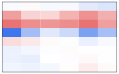
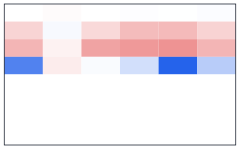
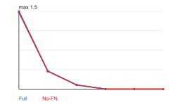
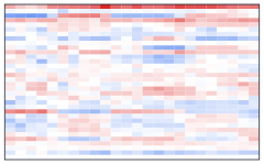
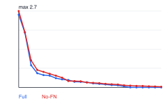
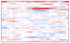
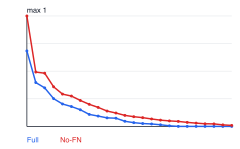
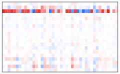
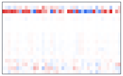
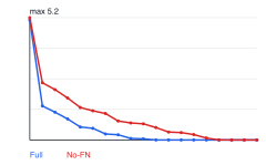
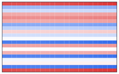
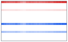
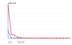
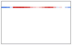
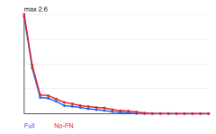
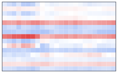
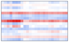
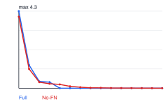
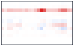
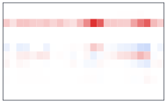
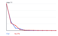
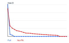
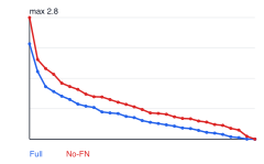
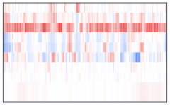
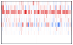
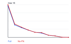
The first ablation grid shows the smaller synthetic and real-world tasks. Each row compares the full objective, the no-row-sparsity variant, the no-temporal-smoothing variant, and the singular-value spectrum used to diagnose the Frobenius/nuclear pair.
| Data set | Full | No row sparsity | No temporal smoothing | Singular values |
|---|---|---|---|---|
| Synthetic | 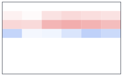 |
 |
 |
 |
| Bike sharing |  |
 |
 |
 |
| Appliances |  |
 |
 |
 |
| Parkinsons | 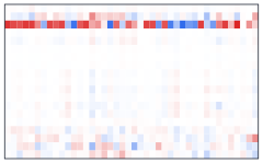 |
 |
 |
 |
| Seoul bike | 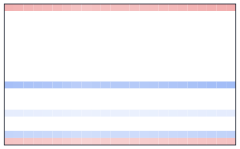 |
 |
 |
 |
| Metro traffic |  |
 |
 |
 |
| Air quality | 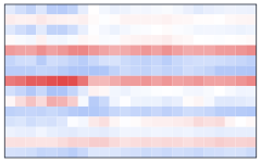 |
 |
 |
 |
| Household power | 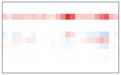 |
 |
 |
 |
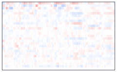
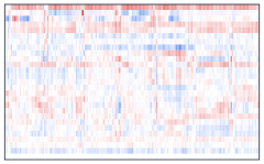
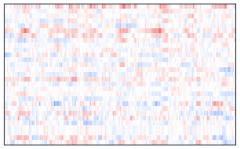
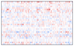
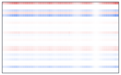
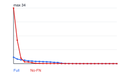
The second grid uses the same panel convention for larger hour-of-week problems with $m=168$ ordered tasks.
| Data set | Full | No row sparsity | No temporal smoothing | Singular values |
|---|---|---|---|---|
| Bike week-hour |  |
 |
 |
 |
| Appliances week-hour | 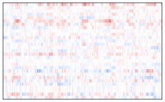 |
 |
 |
 |
| Metro week-hour | 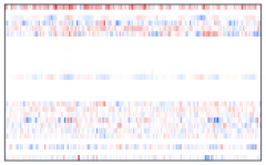 |
 |
 |
 |
| Power week-hour | 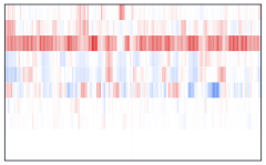 |
 |
 |
 |
The full robust model does not win every data set, which is expected because the usefulness of each structural assumption depends on the data. But the pattern is consistent:
- The robust calibrated loss often improves over the squared-loss variant. In the reported clean test table, the full robust model has lower MSE than the squared-loss version on 9 of 12 data sets. Under added training-response noise, it is lower on 10 of 12 settings.
- The $\ell_{2,1}$ term usually reduces the number of effective feature rows, which confirms its shared feature-selection role.
- The fused term usually reduces temporal roughness, and removing it often hurts temporal data such as Seoul Bike, Metro Traffic, and the larger hour-of-week variants.
- The Frobenius/nuclear pair controls the singular-value spectrum, but its predictive effect is data dependent. In some data sets it helps generalization, while in others it can over-shrink useful task heterogeneity.
The task-order diagnostic is especially important. If temporal smoothness is a real prior, then the true order should beat a random order. The paper finds that randomizing the task order usually degrades the fused model, which supports the use of a path-graph temporal penalty when the tasks are naturally ordered.
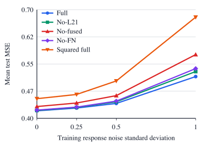
The noise sweep gives a compact picture of the robustness story. As the training response noise increases, the squared-loss version degrades faster than the robust models. The full model has the lowest average MSE across the sweep, with the no-L21 and no-FN variants close behind at lower noise levels.
Takeaways
The main modeling lesson is that robust multi-task regression benefits from separating several kinds of structure. The calibrated residual loss handles heterogeneous noise. The $\ell_{2,1}$ norm asks the tasks to share features. The fused penalty asks neighboring tasks to evolve smoothly. The Frobenius/nuclear pair asks the coefficient matrix to stay controlled and approximately low-rank.
The main optimization lesson is that the nonsquared residual loss is easier to handle in the dual: it turns into simple norm-ball constraints. Once the dual is smooth, accelerated projected-gradient ascent becomes natural, and three-operator splitting gives an efficient way to solve the structured primal subproblem.
For temporal prediction problems, the model is most compelling when the task order is meaningful and noise levels vary across tasks. In that setting, robustness and temporal smoothness are not separate tricks; they work together to produce predictors that are both stable and interpretable.
References
- Rich Caruana. “Multitask Learning.” Machine Learning, 28(1), 41-75, 1997.
- Andreas Argyriou, Theodoros Evgeniou, and Massimiliano Pontil. “Convex Multi-task Feature Learning.” Machine Learning, 73(3), 243-272, 2008.
- Pinghua Gong, Jiayu Zhou, Wei Fan, and Jieping Ye. “Efficient Multi-task Feature Learning with Calibration.” Proceedings of KDD, 761-770, 2014.
- Han Liu, Lie Wang, and Tuo Zhao. “Multivariate Regression with Calibration.” Advances in Neural Information Processing Systems, 27, 2014.
- Robert Tibshirani, Michael Saunders, Saharon Rosset, Ji Zhu, and Keith Knight. “Sparsity and Smoothness via the Fused Lasso.” Journal of the Royal Statistical Society: Series B, 67(1), 91-108, 2005.
- Jun Liu, Shuiwang Ji, and Jieping Ye. “Multi-task Feature Learning via Efficient l2,1-Norm Minimization.” arXiv:1205.2631, 2012.
- Damek Davis and Wotao Yin. “A Three-Operator Splitting Scheme and Its Optimization Applications.” Set-Valued and Variational Analysis, 25(4), 829-858, 2017.
- Ting Kei Pong, Paul Tseng, Shuiwang Ji, and Jieping Ye. “Trace Norm Regularization: Reformulations, Algorithms, and Multi-task Learning.” SIAM Journal on Optimization, 20(6), 3465-3489, 2010.
- Amir Beck and Marc Teboulle. “A Fast Iterative Shrinkage-Thresholding Algorithm for Linear Inverse Problems.” SIAM Journal on Imaging Sciences, 2(1), 183-202, 2009.
- Hadi Fanaee-T and Joao Gama. “Event Labeling Combining Ensemble Detectors and Background Knowledge.” Progress in Artificial Intelligence, 2(2-3), 113-127, 2013.
- Luis M. Candanedo, Veronique Feldheim, and Dominique Deramaix. “Data Driven Prediction Models of Energy Use of Appliances in a Low-Energy House.” Energy and Buildings, 140, 81-97, 2017.
- Athanasios Tsanas, Max A. Little, Patrick E. McSharry, and Lorraine O. Ramig. “Accurate Telemonitoring of Parkinson’s Disease Progression by Noninvasive Speech Tests.” IEEE Transactions on Biomedical Engineering, 57(4), 884-893, 2010.
- UCI Machine Learning Repository. “Seoul Bike Sharing Demand.” 2020.
- John Hogue. “Metro Interstate Traffic Volume.” UCI Machine Learning Repository, 2019.
- Saverio De Vito, Ettore Massera, Marco Piga, Luca Martinotto, and Girolamo Di Francia. “On Field Calibration of an Electronic Nose for Benzene Estimation in an Urban Pollution Monitoring Scenario.” Sensors and Actuators B: Chemical, 129(2), 750-757, 2008.
- Georges Hebrail and Alice Berard. “Individual Household Electric Power Consumption.” UCI Machine Learning Repository, 2006.